Notes on ppviz

ppviz is a web-based visualizer for pping. The capture point (CP) must see the flows of both directions of a stream to record RTTs which are RTT estimates from the CP to a host. There are two versions of ppviz, offline and live. Both use output from pping run with the -m flag. pping outputs a line for every RTD sample it computes, triggered by the arrival of a packet from the pping’d host (inbound to CP) which matches a previously seen (outbound to host) packet of the reverse flow. The -m flag outputs more fields per line, data that can be particularly useful for understanding of the observed RTD values. The pping lines are annotated with the flow in the inbound-to-CP direction (from the pping’d host ) and have the format:

time RTD min [Fbytes Dbytes Pbytes] flow

where:

time: arrival time of triggering packet, inbound to CP from pping’d host

RTT: estimate of RTD between CP and host, for this particular stream

min: smallest value of RTD seen so far

Fbytes: total number of bytes passed outbound from CP to host (collected at arrival of reverse flow at CP)

Dbytes: total number of bytes passed outbound from CP to host (by this flow’s reverse flow) that have departed the CP-to-host side, (collected at arrival of inbound host-to-CP packets that match a stored outbound packet)

Pbytes: number of bytes passed inbound to CP from host on this flow since last RTD sample

flow: string giving flow name in IPsrc:port+IPdst:port format

The xbytes fields can safely be ignored by most users. They let us compute the bytes that this packet sees in the pipe (which we expect to be correlated with delay). Fbytes - Dbytes gives the number of bytes that were ahead of the outbound packet in the CP-to-host direction. Pbytes gives the number of bytes that were ahead of the inbound packet in the host-to-CP direction. The released version of ppviz does not currently use Fbytes, Dbytes, and Pbytes, but their use is under development for future versions and is available for use in your own diagnostics. A picture describing the three optional fields would be helpful and one is likely to appear in the future.

ppviz offline

For offline use, the html file ppvizFF.html is used on saved file of pping output lines. The file is created by running pping with the -m option and saving the output to a file, e.g. ppingEX.txt. The ppingEX.txt file can be created directly from running pping with the -i flag, gathering data on an interface, or by running pping with the -r flag on a pcap file.

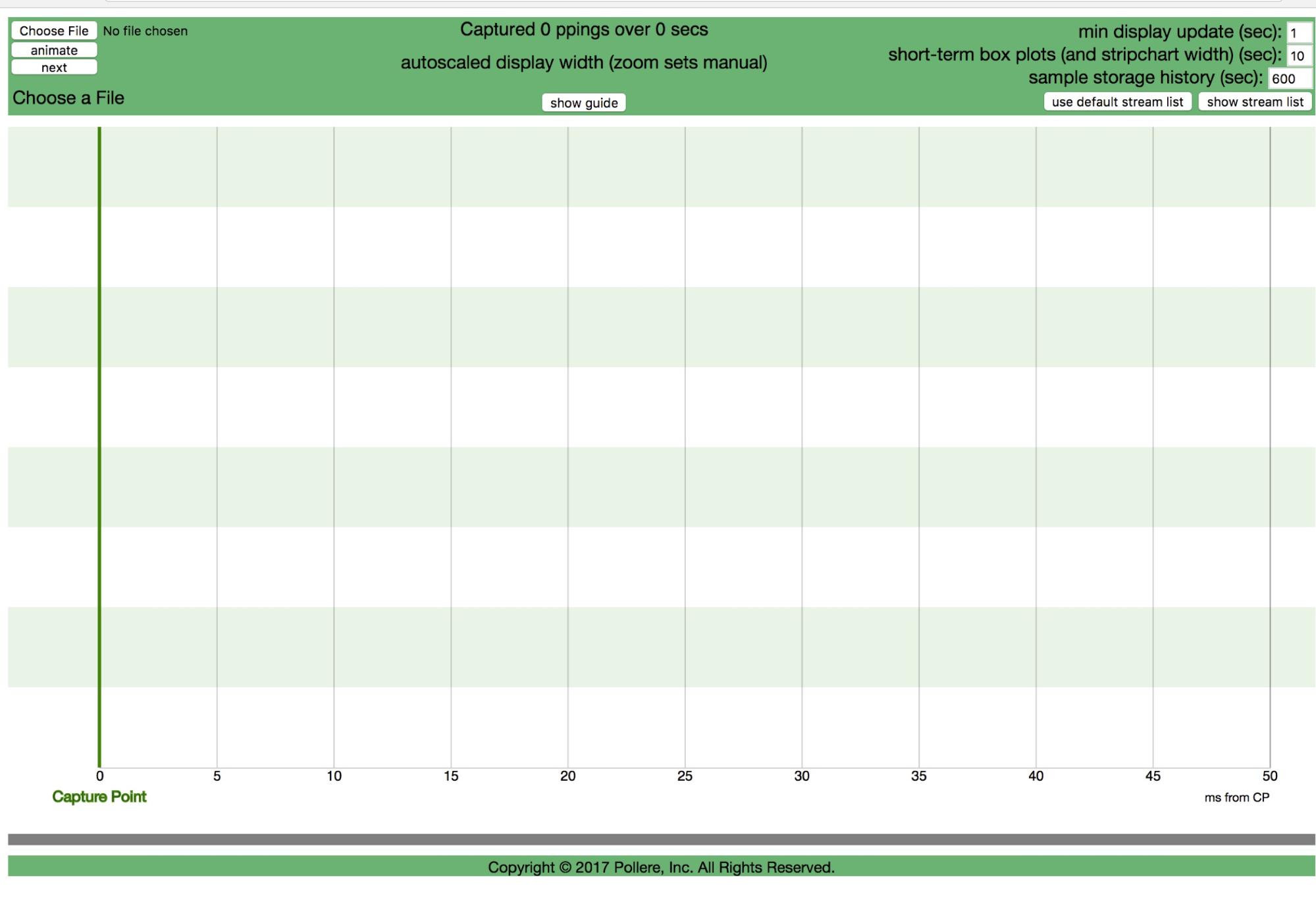
Open the ppvizFF.html file to get the screen shown below. Use the “show guide” button to display a “Guide” text area (it can be removed with the “hide guide” button) that pops up below the gray bar. The area below that can be used for strip charts.

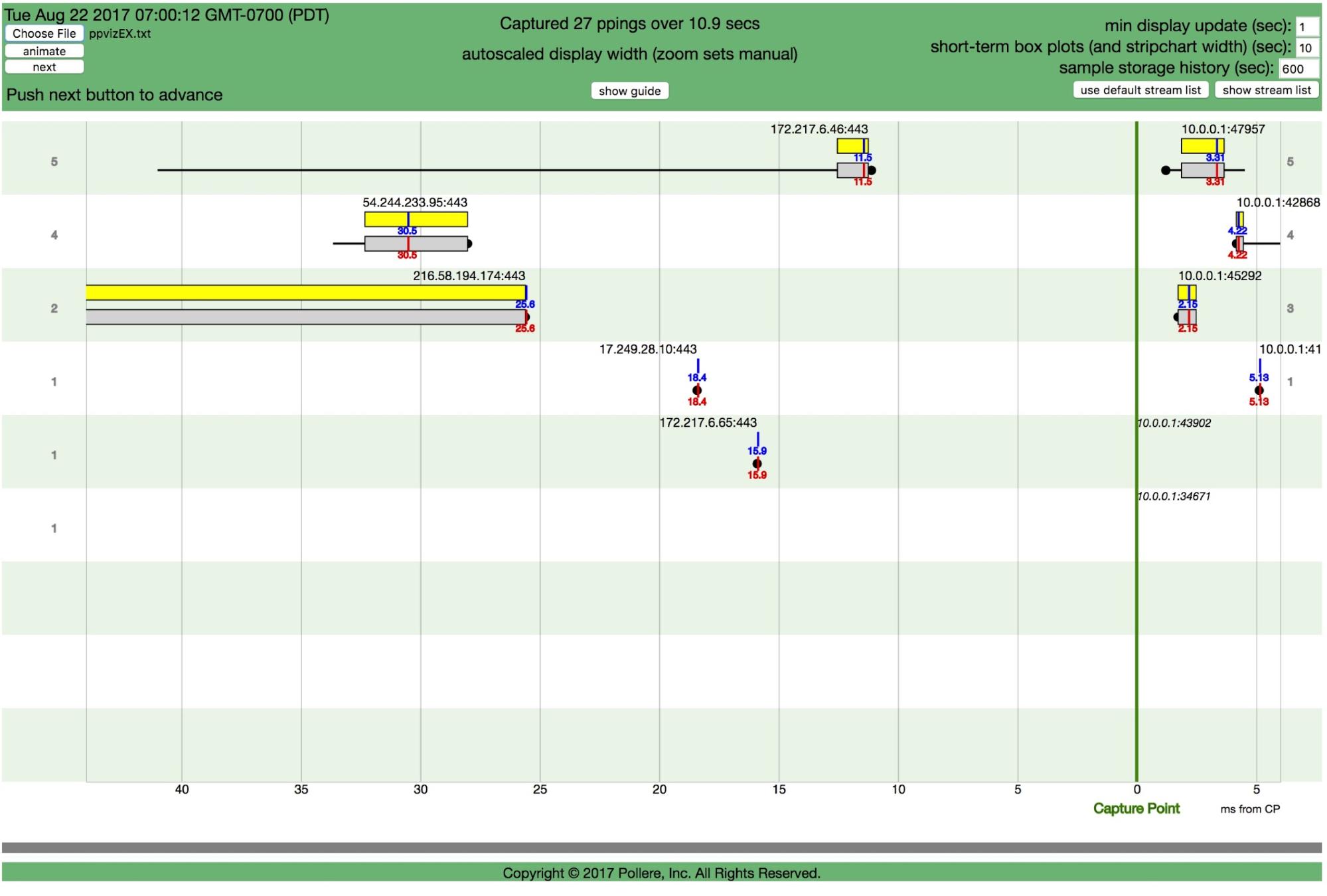
Use the “Choose File” button on the top left to select the input file created with the pping -m command. A sample file, ex.pp, is included in the distribution. The initial display uses box plots to display stream statistics, one stream in each “lane” of alternating colors. If the Capture Point (CP) is inside a network, e.g. a “bump in the wire” or collection process in a network element, each flow of a stream will be displayed on opposite sides of the capture point, in the same lane, as shown here. If no data is available for one direction of a flow, the destination port address is shown in italics on the side of the CP corresponding to its host. Statistics for the recent short-term are shown in yellow boxes that cover the IQR, from 25th to 75th percentile with a blue line showing median value. The length of this short-term history is set on the upper right hand side of the header region, here 10 seconds. Statistics for the full history of a flow are kept using tdigest (https://github.com/welch/tdigest) and are shown in gray boxes (below the yellow), which also have whiskers for 5th to 95th percentile and a large dot for the minimum pping time. The “next” button progresses each statistics update through time; the “animate” button can be used to progress through automatically at 1/10 real time. The gray bar below the statistics display can be grabbed and moved to change the ratio of strip chart area to statistics display area. Sample storage history is the number of seconds of past pping samples kept in memory.

The unix timestamp in the file is used to compute the date and time of capture in the upper left of the green header area. In the example, only six streams were found in the first 10.9 seconds of the trace. This capture point is next to a cable modem (the home IP address was changed to 10.0.0.1 to anonymize). The Internet has ended up on the left side; the home network on the right. The minimum round trip delays to the servers are in the 12 to 27 ms range. Inside the house, the minimums are under 5 ms. There’s not a lot of data at this point.

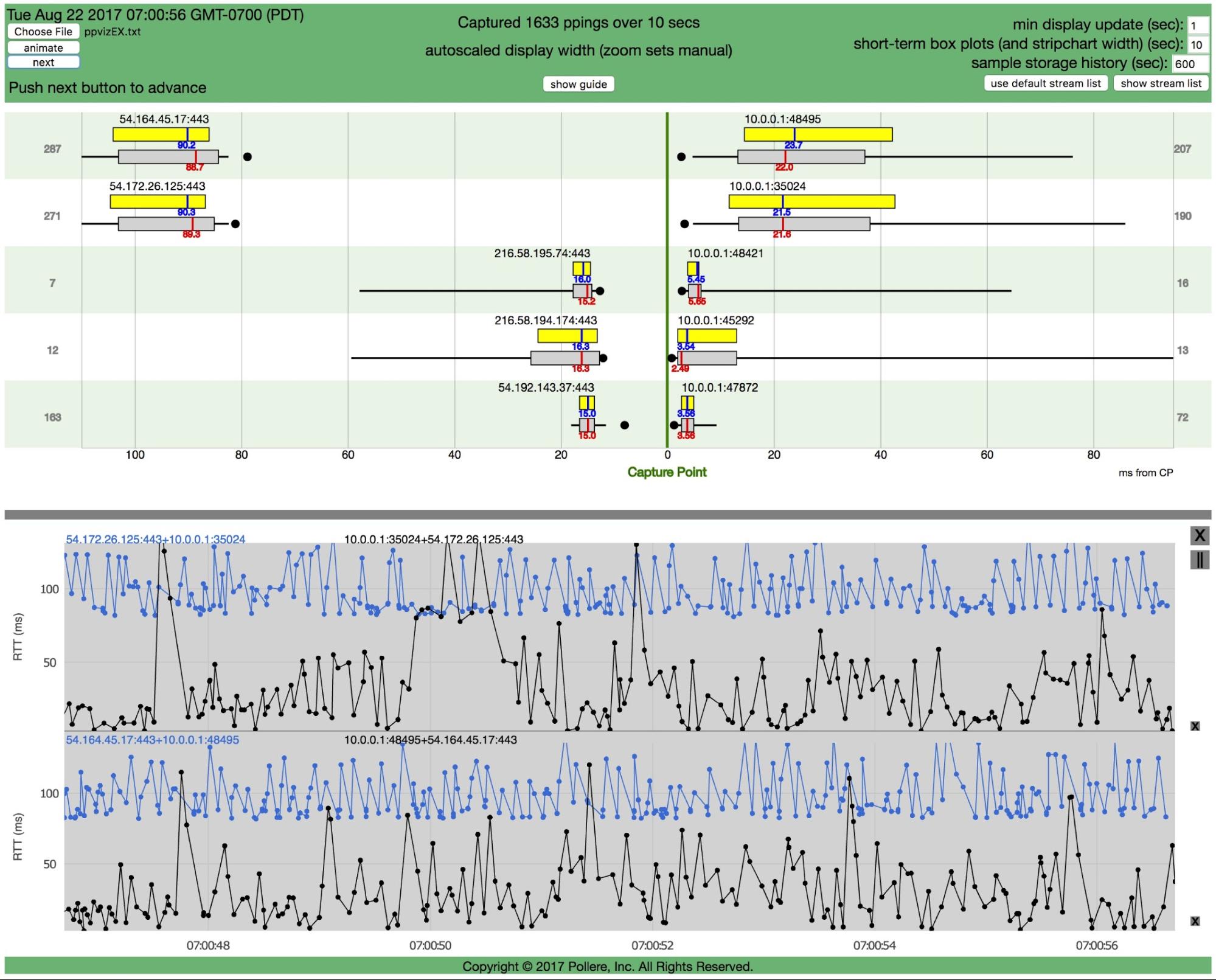
Clicking on a lane creates a strip chart area with a strip chart trace of the flow on that side in that lane. The strip chart area can be closed by clicking on the “X” to the right of the strip chart. Strip charts are updated at the minimum display update (selected in the upper right hand corner of the header) and input can be paused (for analysis) by clicking the pause button below the “X”. Strip charts use plotly.js (https://plot.ly/javascript/) so those analysis tools are available, best used when the strip chart updates are paused. Up to four streams can currently be displayed, the new entries stacking on top of the old. Each stream gets its own closer “X” in the lower right corner of the chart.

It’s clear for this example that the flows to ports 48495 and 35024 are the large, persistent flows (in fact, they are part of a video delivery). Their round trip internet distance from the capture point (the home edge) is +/-80ms and though the minimum round trip delay in the home is small the delay variability is much larger.

Initially streams are chosen for display in the statistics area by largest number of samples in the most recent statistics interval. This can be changed by selecting “show stream list” and selecting which streams you want to see. Go back to a sorted list by selecting “use default stream list”. The width of the statistics display area can be changed by zooming; that setting will persist unless autoscale is selected.

When run from an end host, the end host is the CP so only one side of a stream is shown. The destination IP addresses and port is shown in italics on the opposite side of the CP line for identification of the flow.

ppviz live (still in testing)

For live or online use, ppvizCLI.html reads from a web socket that serves the lines from a pping command running with the -i flag on an interface. Online use is facilitated by bundling all the needed commands. The two interfaces differ slightly in the controls available in the green header region. The web page comes up showing the current date and time in the upper left and will indicate its status (initially “Opening Websocket”). The screen updates according to the values set on the right hand side of the header which are the same as for ppviz offline.

Notes and caveats

Keep in mind that pping produces RTT samples for each flow at roughly the same intervals as the underlying TCP flow produces new TSvals, currently between 1 and 10 ms. This means that some of the “peaks and valleys” of delay can be missed. Additional information can be mined from the packet stream for a more complete picture, specifically the Fbytes, Dbytes, and Pbytes values described above.

ppviz was created with the consumer edge and educational use in mind. Indications are that it can be useful at higher speeds and with higher precision TSvals, but such usage may overtax the underlying open source plotting packages.

This is an open source prototype and improvements are possible and likely (some are in progress). If you decide to make some, please let us know at info@pollere.net. We are particularly interested in improving the selection of flows to display (e.g., “show me all the flows from source 10.0.0.1”). You may report bugs to the same address.